PADM 702 Research Paper: Simple Time Series Analysis Using Exponential Smoothing (Example Report With Chart)
Need help with this assignment?Get an original answer from a qualified tutor — from $10/page.
Get it written →PADM 702 Research Paper: Simple Time Series Analysis (Exponential Smoothing)
Time series analysis lets public administrators and policy analysts examine a variable over equally spaced intervals of time (for example, monthly or yearly income figures), discern patterns and forecast future values. A time series plot reveals (1) outliers and sudden shifts and (2) long-term increases or decreases, and shows whether the pattern is linear or nonlinear. The analyst then asks why.
Following the course’s Simple Time Series Analysis Assignment Guide, compute and interpret a simple time series analysis called exponential smoothing, and write a four-page doctoral-level report stating your findings, including chart(s).
Look for trend, shifts and outliers
Ft+1 = αYt + (1 − α)Ft
MAD, MSE, MAPE and bias
Explain why, forecast, state limits
About the data: the assignment guide and data set were not included in the copy we received, so this model uses labeled sample data for a fictional city. Use the variable and software (Excel, SPSS or R) your guide specifies; the steps and interpretation are the same.
Model research report
Original example for study purposes (about 1,050 words plus a chart and table, roughly four double-spaced pages). The City of Lakeview and its revenue figures are fictional sample data.
Introduction
Local governments depend on revenue forecasts to adopt balanced budgets, and errors in either direction carry costs: overestimates force midyear cuts, while underestimates lead to unnecessary service reductions or tax increases. This report applies simple exponential smoothing (SES) to 15 years of sales tax revenue for the fictional City of Lakeview, fiscal years (FY) 2011 to 2025, to describe the pattern in the series, compare smoothing constants and produce a forecast for FY2026. The report then interprets the results and discusses their implications and limitations for budget decision-making.
Method
Exponential smoothing forecasts the next value as a weighted average of the most recent observation and the previous forecast, so the weights on older observations decline exponentially (Hyndman & Athanasopoulos, 2021). The SES equation is Ft+1 = αYt + (1 − α)Ft, where Yt is the actual value in period t, Ft is the forecast for period t and α is the smoothing constant between 0 and 1. A small α produces a smooth forecast that reacts slowly to change, while a large α reacts quickly but also follows random noise. The method dates to Brown’s (1959) work on inventory forecasting and remains widely used because it is simple and often accurate for short-term forecasting (Gardner, 1985).
The first forecast (FY2012) was initialized with the FY2011 actual value. Forecasts were computed in a spreadsheet for α = 0.2, 0.5 and 0.8, and accuracy was compared with mean absolute deviation (MAD), mean squared error (MSE), mean absolute percentage error (MAPE) and bias (the mean of actual minus forecast) for FY2012 to FY2025.
Results
Time series plot. Figure 1 shows the actual revenue series and the three smoothed forecasts. Revenue rose from $42.1 million in FY2011 to $60.2 million in FY2025, a compound growth rate of about 2.6% per year. The pattern is close to linear, with one clear exception: a sudden drop from $52.8 million in FY2019 to $48.1 million in FY2020, followed by a rapid recovery that brought revenue above its pre-shock trend by FY2022.
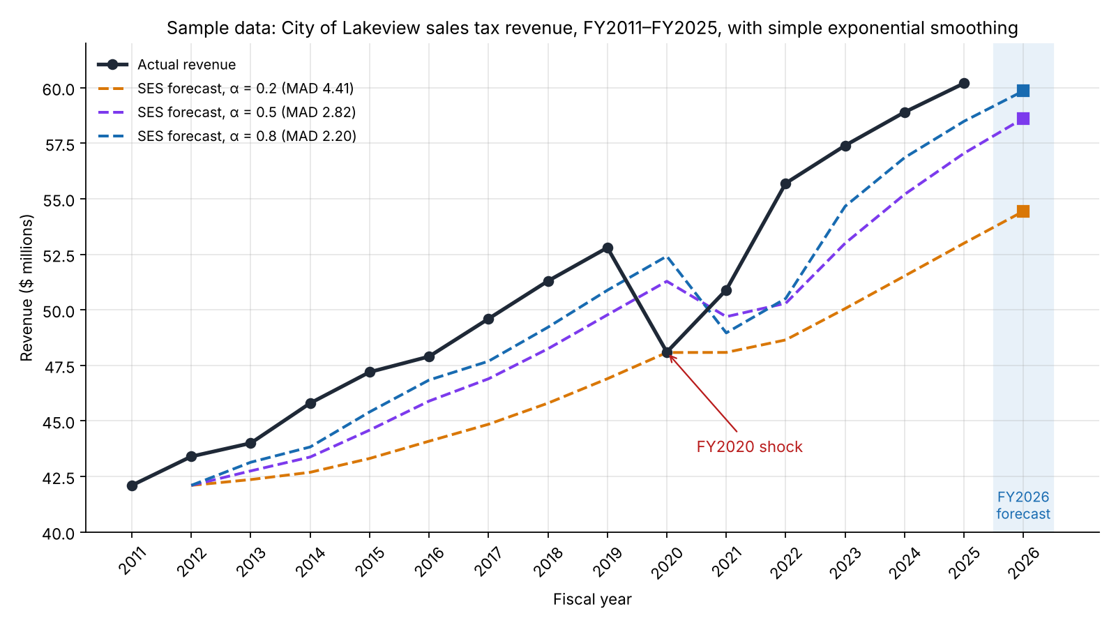
Figure 1. Sample sales tax revenue with SES forecasts and FY2026 projections.
Table 1. Actual revenue and SES forecasts ($ millions)
| Fiscal year | Actual | Forecast α = 0.2 | Forecast α = 0.5 | Forecast α = 0.8 |
|---|---|---|---|---|
| FY2011 | 42.1 | — | — | — |
| FY2012 | 43.4 | 42.10 | 42.10 | 42.10 |
| FY2013 | 44.0 | 42.36 | 42.75 | 43.14 |
| FY2014 | 45.8 | 42.69 | 43.38 | 43.83 |
| FY2015 | 47.2 | 43.31 | 44.59 | 45.41 |
| FY2016 | 47.9 | 44.09 | 45.89 | 46.84 |
| FY2017 | 49.6 | 44.85 | 46.90 | 47.69 |
| FY2018 | 51.3 | 45.80 | 48.25 | 49.22 |
| FY2019 | 52.8 | 46.90 | 49.77 | 50.88 |
| FY2020 | 48.1 | 48.08 | 51.29 | 52.42 |
| FY2021 | 50.9 | 48.08 | 49.69 | 48.96 |
| FY2022 | 55.7 | 48.65 | 50.30 | 50.51 |
| FY2023 | 57.4 | 50.06 | 53.00 | 54.66 |
| FY2024 | 58.9 | 51.53 | 55.20 | 56.85 |
| FY2025 | 60.2 | 53.00 | 57.05 | 58.49 |
| FY2026 forecast | — | 54.44 | 58.62 | 59.86 |
Table 2. Forecast accuracy, FY2012–FY2025
| Measure | α = 0.2 | α = 0.5 | α = 0.8 |
|---|---|---|---|
| MAD ($ millions) | 4.41 | 2.82 | 2.20 |
| MSE | 24.94 | 9.25 | 6.16 |
| MAPE | 8.33% | 5.42% | 4.28% |
| Bias (actual − forecast) | +4.41 | +2.36 | +1.59 |
| FY2026 forecast | $54.44M | $58.62M | $59.86M |
The smoothing constant α = 0.8 produced the lowest error on every measure, with a MAPE of 4.3% compared with 8.3% for α = 0.2. Its FY2026 forecast is $59.86 million. All three models show positive bias, meaning they underestimated revenue on average, and the bias is largest when α is small.
Interpretation
Why the high smoothing constant performs best. SES assumes that the series fluctuates around a level without a persistent trend. Lakeview’s revenue has a steady upward trend, so a forecast built on past values always lags behind; the more weight the model gives to older values, the further behind it falls. A high α keeps the forecast close to the most recent actual value and therefore reduces, but does not remove, the lag. The consistent positive bias is the signature of a trend that SES cannot capture, and it means that every FY2026 forecast in Table 2 is likely too low. If the historical growth rate continued, FY2026 revenue would be about $61.8 million, roughly $1.9 million above the best SES forecast.
Why the FY2020 shift occurred. The sudden decline in FY2020 is an outlier relative to the trend, consistent with an external economic shock such as a recession or public health emergency that reduced taxable retail activity. The rapid recovery in FY2021 and FY2022 could reflect pent-up consumer demand, inflation in taxable prices, federal stimulus or growth in taxable online sales. SES handles such shocks imperfectly: high-α models overreact, forecasting FY2021 revenue near the depressed FY2020 level, while low-α models are slow to recognize the recovery. Analysts should investigate the causes before assuming the post-shock growth will continue.
Implications for public administrators. For budgeting, the α = 0.8 forecast offers a conservative baseline, which some finance officers prefer because underestimating revenue protects against midyear shortfalls. However, systematic underestimation also has costs, such as unnecessary service reductions or larger-than-needed reserves, and it can erode the credibility of the forecasting process with elected officials. A prudent approach is to present the SES forecast alongside a trend-adjusted forecast and a downside scenario that reflects the FY2020 shock, then document the assumptions behind the adopted figure.
Limitations and Recommendations
This analysis has several limitations. First, SES is designed for series without trend or seasonality; for trending data, Holt’s linear method, which adds a smoothed trend term, is more appropriate (Holt, 2004; Hyndman & Athanasopoulos, 2021). Second, annual data provide only 14 forecast errors, so accuracy comparisons are sensitive to the FY2020 outlier. Third, the forecast is purely extrapolative and ignores drivers such as employment, inflation, tax-rate changes and economic development projects. Finally, the choice of initialization affects early forecasts. I recommend that Lakeview (1) adopt Holt’s method or a regression with economic indicators for the official forecast, (2) use monthly data to detect turning points earlier and (3) re-estimate the smoothing parameters each year as new data arrive.
Conclusion
Exponential smoothing shows that Lakeview’s sales tax revenue follows a steady upward trend interrupted by a one-year shock in FY2020. Among the constants tested, α = 0.8 fits best, yet all SES models underestimate revenue because the method does not model trend. Used carefully and supplemented by trend-adjusted methods and scenario analysis, simple time series tools can make revenue forecasts more transparent and defensible for public budget decisions.
References
Brown, R. G. (1959). Statistical forecasting for inventory control. McGraw-Hill.
Gardner, E. S., Jr. (1985). Exponential smoothing: The state of the art. Journal of Forecasting, 4(1), 1–28. https://doi.org/10.1002/for.3980040103
Holt, C. C. (2004). Forecasting seasonals and trends by exponentially weighted moving averages. International Journal of Forecasting, 20(1), 5–10. https://doi.org/10.1016/j.ijforecast.2003.09.015
Hyndman, R. J., & Athanasopoulos, G. (2021). Forecasting: Principles and practice (3rd ed.). OTexts. https://otexts.com/fpp3/
How to compute it in Excel: put years in column A and values in column B. In C3 enter =B2, in C4 enter =$F$1*B3+(1-$F$1)*C3 with α in cell F1, and fill down. Errors are =B3-C3; MAD is the average of their absolute values. Excel’s Data Analysis ToolPak also has an Exponential Smoothing tool, but it asks for the damping factor, which equals 1 − α.
Frequently asked questions
How do I choose the smoothing constant?
Test several values and choose the one with the lowest error (MAD, MSE or MAPE) on past data, or let software estimate the value that minimizes squared error. Then check whether the forecasts are biased.
Why are all my SES forecasts below the actual values?
Your series probably has an upward trend. SES lags trending data, so use Holt’s method or note the bias in your interpretation.
What is the difference between a moving average and exponential smoothing?
A moving average weights the last few periods equally and ignores older data; exponential smoothing uses all past data with weights that decline exponentially.
More model assignments posted today
Get a plagiarism-free answer to this question
Send us your instructions and we’ll match you with the best writer in your subject.
- 100% human-written, zero AI
- Turnitin report included
- Confidential — we never share your data
- Free revisions & refunds